How-To Guides

MuirWave opens in nautical-chart conventions (feet, nautical miles, DMS, knots). There are two ways to change that, and they write the same setting.

1. Open Settings from the home screen, then Units
   Six rows: depth, range, coordinates, speed, temperature and sound speed.
2. Tap the option you want
   Every option for that quantity is on screen, so there's no cycling to find one. The full name of your choice appears under the row.
3. The whole app follows immediately
   Every readout, chart axis, map label and chip switches at once — and stays switched across relaunches, Reset, and opening someone else's project.

1. Tap the readout itself
   Most depth, range, coordinate and sound-speed readouts cycle on tap — feet → metres → fathoms → back to feet; coordinates DMS → DDM → DD. Quicker when you're looking at the number and just want the other unit.
2. It's the same setting
   Cycling a chip changes the same preference the Settings card shows, so the two can never disagree.

MuirWave separates two jobs so you never confuse "what are conditions here" with "what does my source do". Both live on the map.

You dropped a bathythermograph and the layer is at 600 ft; the model says 164 ft. Type what you measured and every prediction rebuilds through it — measured truth beats modelled truth. Free for everyone, works fully offline.

1. Open the Water Column panel
   From the panel rail (OCEAN group), open Water Column and find the MEASURED LAYER · BT/XBT OBSERVATION block. It's there with or without a regional pack.
2. Enter your sonic layer depth
   Tap the Measured SLD row and type the depth you observed (any depth unit — tap the unit chip to switch). The row records when and where you entered it.
3. Flip USE MEASURED on
   The sound-speed profile rebuilds: well-mixed from the surface to your depth, then a smooth splice into the model's structure below. The BELOW LAYER row names exactly what it splices into — live model or climatology, whichever is really underneath.
4. Read the chip
   The top-bar SSP chip turns solid brass with a ◆ glyph — ◆ SSP · MEASURED · <1 H. That look means your observation is driving the solver. The Propagation panel shows both curves: your measured profile bright, the model dashed for comparison.
5. Revert any time
   Toggle USE MEASURED off — or tap the chip and choose REVERT TO MODEL — and the model answer returns instantly. Your entry is kept for one-tap re-enable.

Your display says the noise floor is 74 dB at 400 Hz; the model says 70.7. Enter a handful of points and the modelled spectrum warps through your measurements, re-anchoring the noise level and the whole detection picture. Also free.

1. Open the Ambient Noise panel
   From the panel rail (OCEAN group, just below Currents), open Ambient Noise and scroll to MEASURED NOISE · FIELD OBSERVATION.
2. Add your points
   Tap ADD POINT, enter a frequency and level in the fields that open, then tap SAVE POINT. Up to 12 points; one is perfectly valid. Levels are omnidirectional spectrum level, dB re 1 µPa²/Hz — mind the unit traps in Troubleshooting.
3. Flip USE MEASURED on
   The noise total anchors to your points. The component rows dim ("model breakdown · total is measured-anchored") and the TOTAL row wears a brass MEASURED tag with the model's number kept in fine print — the disagreement is your field intelligence.
4. Watch the fade
   Your points govern within one decade of frequency on either side; beyond that the model honestly takes over. On the spectrum chart your points are brass diamonds the anchored curve passes through; the model total stays dashed underneath.

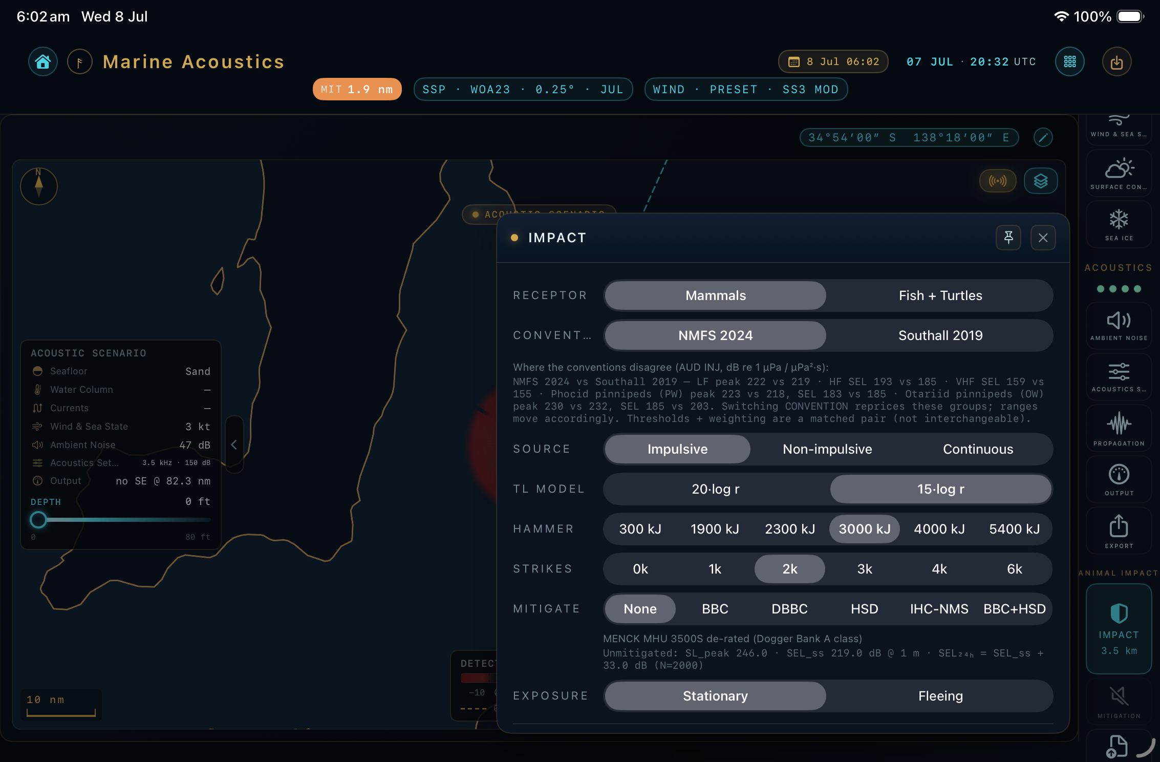
The Impact Ranges panel estimates how far your source could affect marine life, judged against recognised regulatory thresholds — the core of an impact assessment.

1. Drop the pin on your site
   Only the map pin matters here — impact work is self-contained and takes nothing from Acoustics Setup. You never need to open the acoustics scenario for an impact assessment.
2. Open the Impact Ranges panel
   From the panel rail, open Impact Ranges (in the ANIMAL IMPACT group).
3. Choose your receptor & source type
   Pick mammals or fish/turtles, then the source type: impulsive (pile driving, airguns), non-impulsive (vibratory piling, drilling), or continuous (turbines, shipping). These select the correct threshold family.
4. Describe the source in the panel
   The panel's numbers are driven entirely by its own source description: hammer energy and strike count for impulsive sources, or source level and frequency otherwise. Source depth defaults to AUTO (mid-water at the pin — the published pile-driving convention); override it in the panel if you know the real depth.
5. Set the hearing-group convention
   In the panel, choose the hearing-group convention — NMFS 2024 or Southall 2019. This sets which species-group thresholds are used.
6. Set your jurisdiction (in Settings)
   The Compliance Jurisdiction (Settings) — NMFS, BSH, JNCC, EPBC or Southall — frames the assessment for your regulator. All share the NMFS 2024 / Southall 2019 base thresholds, but some (e.g. BSH, JNCC, EPBC) layer additional criteria on top, which the panel and export reflect.
7. Read the ranges
   MuirWave returns the distance at which each threshold (injury / behavioural) is reached, per hearing group — shown as ranges and on the map.

Every export in MuirWave — scenario reports, impact-assessment PDFs, and the raw data and figures behind them — comes from one Export sheet, in two sections: REPORTS and DATA & FIGURES.

1. Finish your scenario or your impact assessment
   Make sure the prediction, or the Impact Ranges panel's source description, reflects what you want to report — the export captures the current state, nothing more.
2. Open the Export sheet
   Two rail tiles reach it: Export (Acoustics group) opens on REPORTS; Export Data & Figures (Animal Impact group) opens on DATA & FIGURES. It's one sheet either way — scroll to reach the other section.
3. Pick a tile, confirm and share
   Tap a format tile, then Export…. MuirWave renders it and hands it to the share sheet (or a save panel on Mac) — save it, email it, or drop it into your report.

MuirWave ships with global-coverage data. For a survey area you care about, a high-resolution regional pack sharpens the ocean climatology behind your predictions.

1. Open your data sources
   Go to MuirWave Settings from the home screen, then pick a source under DATA SOURCES in the sidebar, to see the available regions and what's installed on your device.
2. Pick a region and tier
   Each region offers two tiers — Compact (smaller) and High Quality (finer depth resolution). Choose based on how much detail and storage you want.
3. Download
   Tap to download. Once installed, that region's data is used automatically for any pin inside it — including fully offline.
4. Manage storage
   Remove a pack any time to free space; it's always re-downloadable. Packs don't count against your iCloud backup.

There's nothing to switch on — MuirWave is offline-first. Every prediction runs on data bundled in the app. This matters most at sea, where you'll often have no signal.

1. Before you sail
   While you still have a connection, download any regional packs for your area (Live). Everything else is already on the device.
2. At sea, just work
   Place pins, run predictions, read results — all of it works with the network off, anywhere on Earth.
3. Trust the labels
   The live-data chips will show they're on the built-in climatology baseline rather than a live feed. MuirWave never silently guesses — you always know the provenance of a number.

The full prediction engine is free. Two optional upgrades add live data (MuirWave Live) and professional export (MuirWave Pro) — see the editions matrix for exactly what each includes.

1. Tap the dimmed feature
   Tapping any greyed-out control — a live chip, a pack, or an export tile — opens a screen explaining what it unlocks and the current price.
2. Purchase through the App Store
   MuirWave Live is a subscription (with a free trial); MuirWave Pro is a one-time purchase you own forever. Both go through your Apple ID.
3. Already own it?
   Use Settings → Restore Purchases on a new device — see Troubleshooting → Restoring a purchase.