Tutorial · About 10 minutes
Your First Prediction
We'll run one complete prediction together — from a blank map to reading a convergence zone. Follow along in the app; every step says what you'll see. By the end you'll understand the whole flow, and every other feature is a variation on it.
Before you start. Nothing here needs a subscription or a connection — the free, offline engine runs this whole tutorial. We'll use a deep-water spot in the North Pacific (20° N, 150° W) as a worked example because it shows convergence zones nicely, but any deep location works.
§01
Place your source
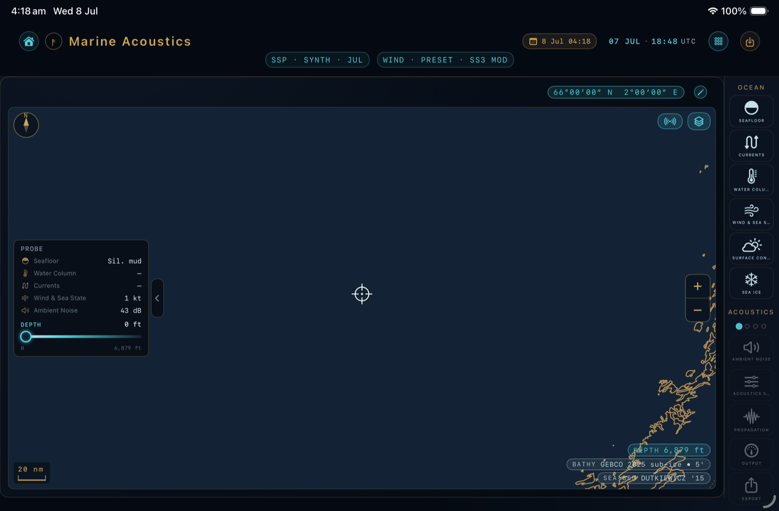
- Open the mapLaunch MuirWave and open the Underwater Acoustics page. The movable cursor you see is the Probe — MuirWave's default. It scouts conditions; it doesn't run a prediction on its own (more on the Probe vs Source split).
- Switch to an acoustic scenarioTap the acoustic-scenario button ("place a source and receiver"). This drops your acoustic Source — the thing making noise — and a receiver onto the map.
- Position the SourceDrag the Source to our example position, roughly 20° N, 150° W — open ocean, well away from the coast. As you settle it, MuirWave pulls the seabed depth, sediment and sound-speed profile for that spot; the bottom-right readout shows the water depth beneath you.
§02
Describe your source
- Set the frequencyUse the frequency slider to choose your source's frequency — try 1 kHz to start. The slider is a smooth log scale from 10 Hz to 50 kHz, so you can set any value, not just fixed steps.
- Set the depthsSet the source depth — how deep the source sits (say 50 m) — and the receiver depth you're listening at. Depth strongly affects which ray paths form.
- Set the source levelSet how loud the source is (its source level). This is the "how loud it starts" term of the sonar equation.
MuirWave assumes no defaults. It waits until you've actually set the frequency, both depths and the source level — it marks which inputs are still needed — and only then runs the prediction. That's why the results appear the moment your scenario is complete, not before.
§03
Read the ray paths
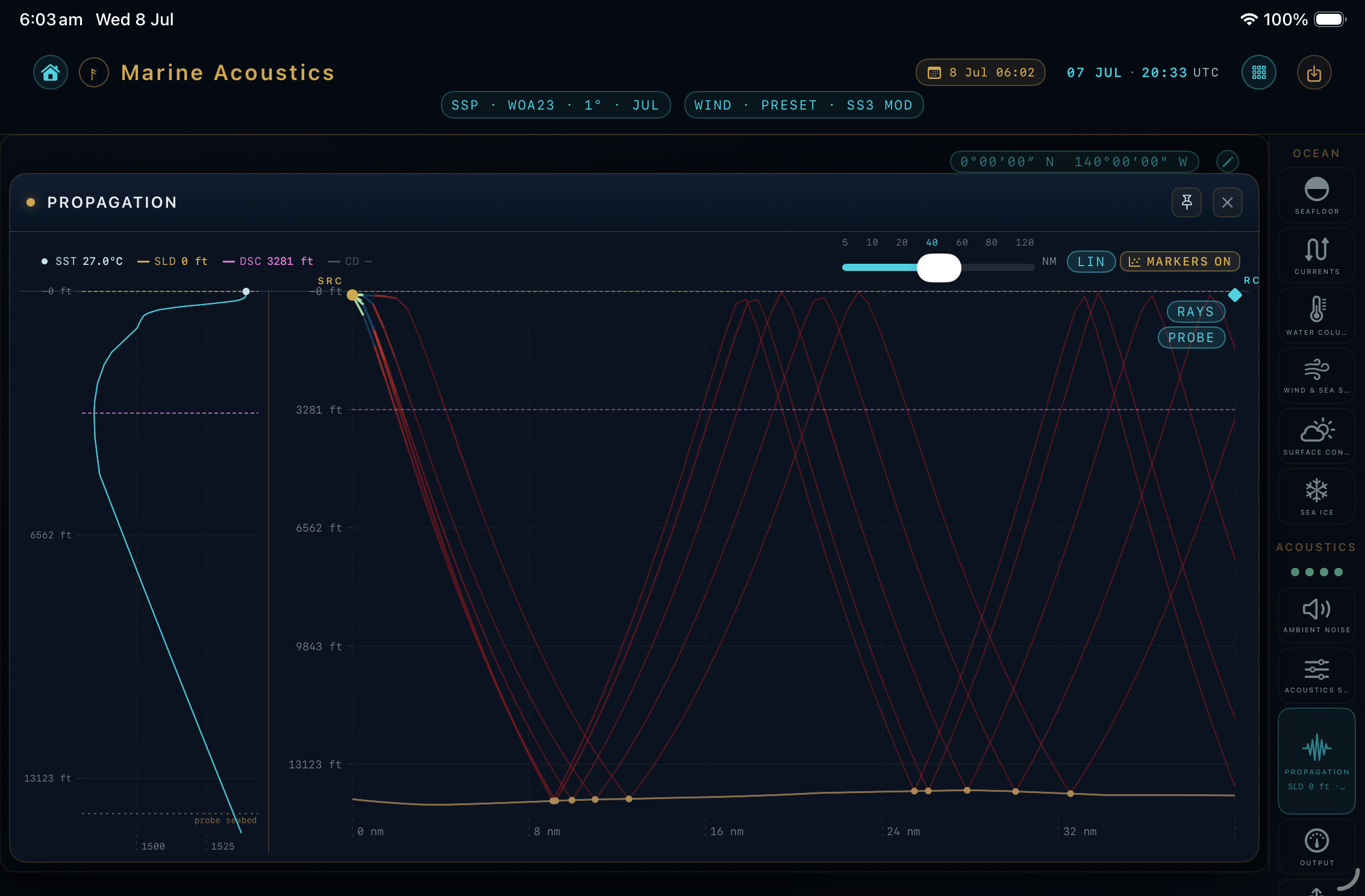
- Open the Ray Path plotThe Ray Path view draws how sound leaves your source and curves through the water — a cross-section from the source outward.
- Spot the convergence zoneFollow the rays: they spread, thin out into a shadow zone, then refocus into a convergence zone (CZ) where sound is loud again. MuirWave marks the first CZ and its range.
- Try the field viewSwitch the plot to FIELD (or BOTH) to see the same information as a continuous picture of where sound reaches. New to this? See Concepts → rays & convergence zones.
§04
Read the answer
- Check Depth ExcessIn the Profile panel, the Depth Excess readout tells you whether the water is deep enough for reliable CZ propagation — and colours itself green / yellow / grey accordingly (what the colours mean). In our deep-water example it should be healthy.
- Read detection / transmission lossThe readouts show how the sound weakens with range and how far it stays detectable. This is the sonar equation resolved for your scenario.
- Change one thing & watchDrag the frequency up to 10 kHz and watch the prediction change — higher frequencies are absorbed faster, so ranges shrink. This live feedback is the fastest way to build intuition.
That's a complete prediction. You placed a source, described it, and read how its sound travels and how far it carries — all offline, from public-domain ocean data.
§05
Where to go next
NEXT
Estimate impact ranges
Turn your prediction into an assessment — how far the source could affect marine life, against regulatory thresholds.
Open the recipe ›
UNDERSTAND
The concepts, explained
Why sound bends, what transmission loss really is, and where convergence zones come from — in plain language.
Read the concepts ›
DO MORE
All the how-to recipes
Regional packs, working offline, the methodology export, changing units, and unlocking Live & Pro.
Browse how-tos ›