Concepts Explained
You don't need an acoustics degree to use MuirWave — but understanding these five ideas makes every readout obvious. Read it once and the numbers stop being mysterious. No maths required; the app does that.
The one idea underneath everything
All of underwater acoustics is really a single question: a sound starts out at some loudness, weakens as it travels, and competes with background noise — can it still be heard? That balance is the sonar equation, and every panel in MuirWave is one term of it.
MuirWave computes each term from the real ocean at your pin. The rest of this page explains the two that do the heavy lifting: transmission loss (how the sea bends and weakens sound) and the sound-speed profile (why it bends the way it does).
The sound-speed profile — why sound bends
Sound doesn't travel in straight lines underwater. Its speed changes with depth — warmer, shallower water carries sound faster; cold deep water slower; then pressure speeds it up again very deep. Sound rays always bend towards slower water, so this profile shapes where sound goes.
MuirWave builds this profile at your pin from ocean climatology (or live data, with MuirWave Live). It's the single most important input — change the profile and the whole prediction changes. The Water Column panel shows it for any spot.
Where the profile comes from — and what Live changes
Drop a pin anywhere in the ocean and MuirWave always has a profile — it ships with global climatology built in, so it works offline, worldwide, with no subscription. MuirWave Live layers real-time ocean data and high-resolution operating areas on top. The app uses the best source available and tells you which one on the SSP chip at the top of the Acoustics screen.
Measured beats modelled
Models are the best guess available before you sail. Once you're on station with a bathythermograph or a live noise display, you have something better — and MuirWave treats it that way.
Enter a measured layer depth or measured noise points and they outrank every model tier — live feed included — for as long as you keep them switched on. The model keeps running underneath (live data keeps fetching, the comparison curves stay on the plots), so reverting never lands you on stale data, and the gap between model and measurement stays visible: that disagreement is field intelligence, not an error to hide.
Transmission loss, rays & convergence zones
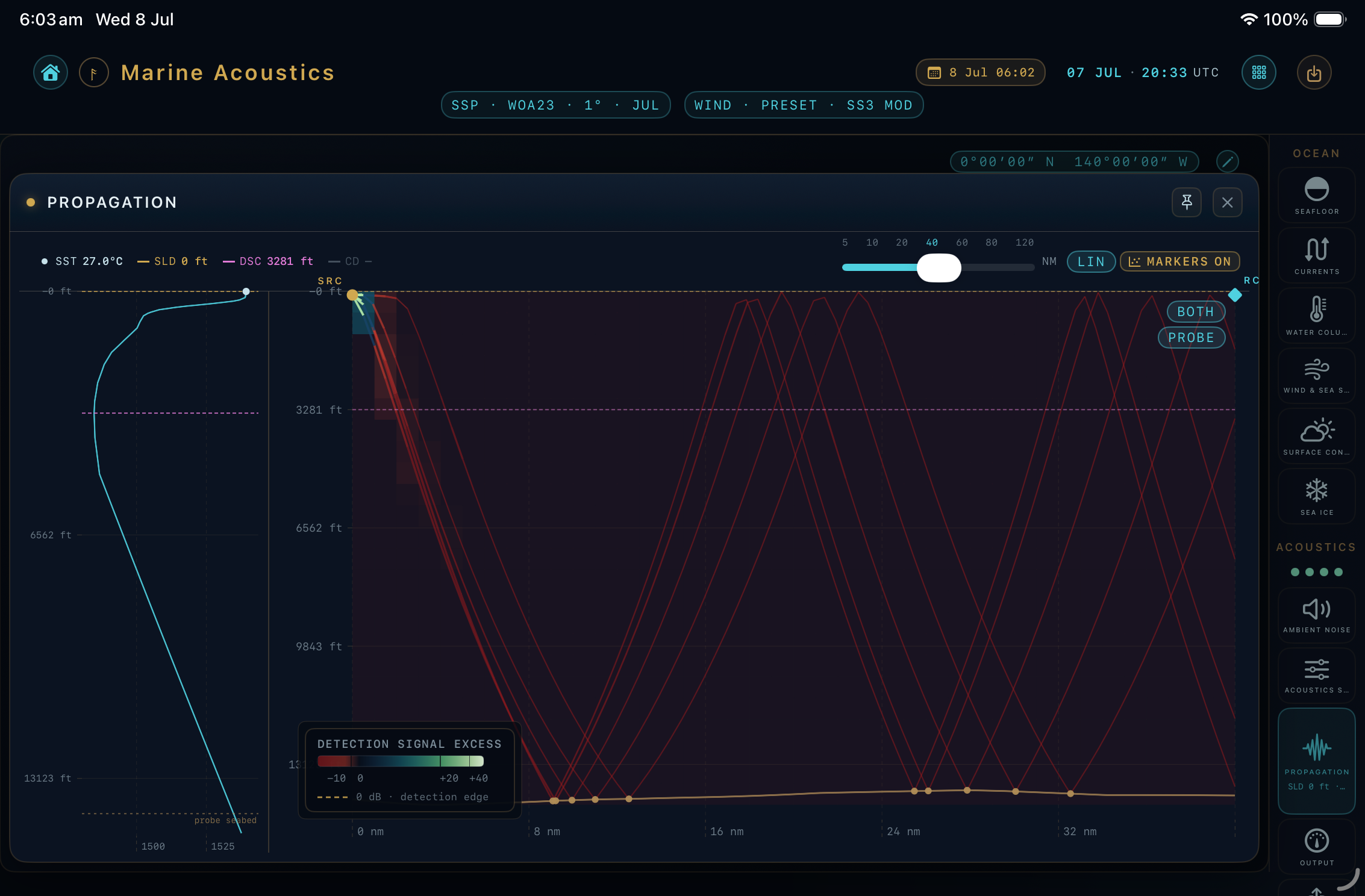
Transmission loss (TL) is simply how much a sound has weakened by the time it reaches a given point — bigger TL means quieter. Because rays bend (§02), sound doesn't fade smoothly: it focuses in some places and thins out in others.
Detection & the sound field
Put the loudness, the loss and the noise together and you get how detectable a source is at each point. MuirWave can paint this across the map as a field — a bird's-eye view of where a source would and wouldn't be heard.
On the Ray Path plot you can switch what's drawn: RAYS shows the ray paths, FIELD shows the continuous detection/loss field, and BOTH overlays them. The structure of the field comes from transmission loss; its overall level comes from the source and receiver you set.
Impact thresholds
For assessment work, the question flips: instead of "can I hear it?", it's "how far out could this sound affect an animal?" Regulators define thresholds — sound levels above which injury or a behavioural response is expected — that differ by species hearing group and by whether the sound is impulsive or continuous.
Where do the thresholds come from?
MuirWave uses the recognised criteria: NMFS 2024 or Southall et al. 2019 (selectable) for marine mammals (grouped by hearing sensitivity) and Popper et al. 2014 for fish and sea turtles. The exact values used appear in your export.
What's an "impact range", then?
The distance from your source at which the received level drops below a given threshold. Inside that range the threshold is exceeded; outside it isn't. MuirWave computes one per threshold and hearing group — see the how-to.
Why does source type matter so much?
MuirWave distinguishes impulsive (pile driving, airguns), non-impulsive (vibratory piling, drilling) and continuous (turbines, shipping) sources — each is judged against a different threshold family, and accumulation over time is handled differently. Setting this correctly is essential for a defensible number.
Why does a fish or sea-turtle row sometimes show a rating instead of a range?
Popper 2014 doesn't publish a numeric threshold for every combination of hearing group, severity and source type. Where it publishes a quantitative dB value, MuirWave computes a real isopleth — a ring on the map, a range in the table. Where it publishes only a qualitative relative-risk rating — near-field / intermediate / far-field, each rated Low / Moderate / High — MuirWave reports that rating instead of inventing a number the standard doesn't provide. Sea-turtle recoverable injury and TTS are the clearest case: Popper rates both qualitatively, so that's what MuirWave shows, never a number borrowed from a fish row.
What about continuous noise — turbines, shipping?
For most fish groups Popper's continuous-noise criteria are qualitative too. One group is the exception: fish whose hearing involves the swim bladder have two published numeric criteria for continuous exposure — 170 dB re 1 µPa (rms) for 48 hours (recoverable injury) and 158 dB rms for 12 hours (TTS) — and MuirWave computes both as real isopleths. The duration is Popper's own exposure assumption, carried through to your export as a label, not something MuirWave models: the range marks where the received level falls to that rms threshold, not a dose accumulated over an animal genuinely staying there 48 or 12 hours. No other fish group, and no source type besides continuous, carries these two numbers.
Globe daylight
The globe's base land and sea follow the selected UTC date and time. Turning the camera does not move geographic sunlight. NOW keeps the light advancing with the existing minute refresh.
Day and night styling fades away as you zoom into the flat chart. Scientific layer colours and legends keep their meaning throughout; decorative lighting does not change a propagation prediction.
Console workspace size
Use the browser console in portrait on phones and in landscape on tablets and larger screens. Tablet workspaces need at least 768 CSS pixels of width; desktop windows need at least 960 CSS pixels and must be at least as wide as they are tall. A rotate or widen message pauses access when the workspace does not fit.
Your scenario, selected chart reading and controls stay in place. Rotate or widen the window to continue where you left off. Opening the keyboard does not change the orientation requirement. After rotating back, tap a field to resume typing; touch keyboards do not reopen automatically. A narrow tablet split view still needs a wider landscape workspace. Sign-in and account recovery remain available from the message.
Inspecting web console charts
In Water Column, touch or hover over the plot to read depth, temperature, salinity and sound speed. The reading stays above the plot after you move away. In Ambient Noise, the frequency reading stays below the Wenz chart. Focus either chart and use arrow keys, Home or End to inspect with a keyboard.
Changing display units retains the selected depth. A changed profile clears its old reading. Wenz shows the four analytic terms and their spectral-density total separately from measured or solved noise; missing shipping data leaves the analytic total unavailable. Inspection reads the displayed data and does not run a prediction.
Web console propagation model
The web console uses an approximate GB7 intensity model. Its prediction, map, 3D field and exact cursor share the same propagation policy and supplied environment. FULL and DIRECT change the displayed extent; they do not change the physical horizon or integration step.
Phase interference and a complete arrival census are not modelled. Map cells and their interpolation approximate sampled intensities. Pending calculations and unsupported paths remain unavailable. A 3D source-depth preview has its own field; Reset returns to the committed scenario.
Radar comparison map
Open RADAR MAP in the forecast field tray to compare the smoothed one-way propagation factor with a standard atmosphere. The map uses a local aircraft antenna height from 50 to 10,000 feet. Its target height is independent; changing it reads the retained field. The other radar panels keep their own platform settings.
Every direction uses the same source atmospheric profile. Land and terrain are unmodelled, and the smooth-sea model includes editable profile assumptions. Colours show stronger or weaker propagation than the standard reference; they do not show detection reach or recommend an altitude. Ranges within ±3 dB have no wash. Missing cells and unsupported polar or globe-edge footprints stay masked.